Compared to traditional disclosure control¶

The methods below are what statistical agencies actually use, applied by experienced people under real constraints. This page is not a league table, and most of these techniques are not competing with this library for the same job.

They mostly solve a different problem

Suppression, rounding and barnardisation are tabular methods: they protect counts in a published table. This library is a per-record mechanism: it changes a value in microdata. The useful comparison is therefore not "which is better" but what does each one guarantee, and against which adversary. Targeted record swapping is the closest relative, because it is the one that also perturbs records.

At a glance¶

	applies to	formal guarantee	holds against auxiliary knowledge	tunable	deterministic
Truncation / generalisation	records	none	no	three settings	yes
Small-number suppression	tables	none	no	threshold only	yes
Random rounding / barnardisation	tables	none	no	base only	no
Targeted record swapping	records	none	no	swap rate	no
This library	records	ε·d̃-privacy	yes	continuous ε	keyed

The column that matters is the middle one, and it is the reason the formalism exists.

What epsilon is "equivalent" to truncating a postcode?¶

A fair question with no exact answer, and the reason is the point. Truncation is not differential privacy, so no \(\varepsilon\) makes the two the same object: truncation releases a fact with certainty, and offers no deniability at any crowd size. Equivalence can only be stated under a chosen yardstick.

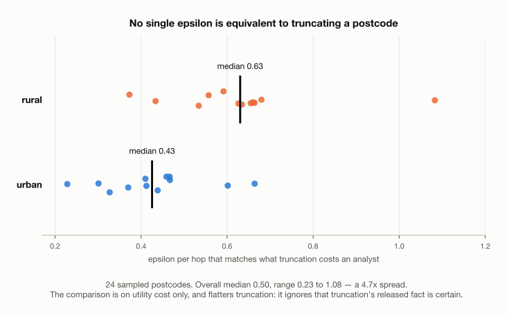
The yardstick used here is what an analyst loses. Told only the outward code, their best guess is a postcode drawn from that district, so their expected error is the population-weighted mean distance from the truth to such a postcode. The equivalent \(\varepsilon\) is the one at which the mechanism displaces people about that far.

Measured over twenty-four sampled postcodes on the August 2026 build:

	min	median	max	spread
urban	0.228	0.426	0.664	2.9×
rural	0.373	0.630	1.083	2.9×
overall	0.228	0.501	1.083	4.7×

So \(\varepsilon \approx 0.5\) per hop costs an analyst about what truncation costs them — on average. Locally it ranges from 0.23 in Stoke-on-Trent to 1.08 in Dundee, because what truncation destroys varies from 0.9 km of positional accuracy in a dense Birmingham district to 16.4 km in a sparse Shropshire one.

Strip plot of equivalent epsilon for urban and rural postcodes

These numbers were re-measured

An earlier version of this page gave an overall median of 0.463 from a spread of 5.3×. Those values were computed on a graph in which Northern Ireland was mistakenly placed in north-west England, which corrupted the neighbourhoods of the sampled postcodes nearest that area: rural Shropshire moved from 0.205 to 0.664 once the coordinates were fixed. The figures above are from the corrected graph.

This comparison flatters truncation

It equates the two on utility cost only. It says nothing about privacy, and every available yardstick is generous to truncation in the same way: all of them ignore that its released fact is certain, and that for nine districts it discloses the postcode unit exactly. Do not read \(\varepsilon = 0.46\) as "truncation is worth \(\varepsilon = 0.46\) of privacy". It is not worth any \(\varepsilon\), because it is not that kind of thing.

Small-number suppression, and why differencing defeats it¶

The standard move is to withhold any cell below a threshold — commonly five or ten. It looks safe: no small count is published, so no individual stands out.

It fails when the margins are published too, which they almost always are, because the suppressed value can simply be recovered by subtraction.

Residents by condition, Ward 7        published        suppressed
  Condition A                               42
  Condition B                               17
  Condition C                                *         <- withheld, below 5
  ------------------------------------------------
  Total                                     62

  62 − 42 − 17  =  3          the suppressed cell, recovered exactly

Nothing was broken into. The published table gives the answer by arithmetic, and protecting against it requires complementary suppression — withholding further, innocent cells purely to break the arithmetic. Doing that consistently across many overlapping tables is a hard combinatorial problem, and getting it wrong is silent.

This is the general shape of the failure. Traditional disclosure control reasons about each release in isolation; an attacker reasons across every release at once, and across whatever else they already know.

Figure to come

An illustration of the same attack across two overlapping geographies, which is the realistic version and harder to see by eye than the single-table case above.

Random rounding and barnardisation¶

Counts are perturbed to a base — rounding to the nearest 3 or 5, or adding small random noise — so that no exact small count is published. This is genuinely a perturbation method and shares some intuition with differential privacy.

What it lacks is an accounting. There is no statement of how much an attacker learns from one table, no way to add that up across many tables, and no parameter to trade against. Averaging many rounded releases of overlapping populations recovers the underlying counts, and nothing in the method bounds how fast.

Targeted record swapping¶

Used by ONS for the 2021 Census: a proportion of households are swapped with similar households elsewhere, with higher rates for records that look risky. This is the closest relative of what this library does — it perturbs microdata, it is randomised, and it is targeted at the records that most need it.

The difference is again the guarantee. The swap rate is a policy choice rather than a privacy parameter, and there is no statement of the form "an attacker's belief changes by at most this much". Swapping also preserves the national totals exactly by construction, which is an advantage this mechanism does not offer.

Why the guarantee is worth the trouble¶

Every method above protects against an attacker the designer imagined. A differential privacy guarantee bounds the likelihood ratio whatever else the attacker knows — before, during or afterwards — and that property is what the formalism was invented for.

The canonical demonstration that traditional control under-protects at scale is the reconstruction work carried out on the 2010 United States Census, which recovered a large fraction of individual records from published tables and prompted the Census Bureau's move to differential privacy for 2020.

Read before citing

The US Census reconstruction result is summarised here from secondary knowledge and has not been checked against the primary sources. It should not be quoted from this page until it has been.

Where this library is the wrong choice¶

You need exact national or regional totals. Swapping preserves them; this does not.
District-level geography is sufficient for your analysis and you have no adversary model worth the name. Truncation is simpler and has no key to lose.
You are publishing tables rather than records. This is the wrong tool entirely; you want a central differential privacy mechanism, which is a separate problem.